Forecasting Data with SARIMA

1. Introduction

I was tasked with forecasting a specific request for the coming quarters using Machine Learning. Since the demand in this case is seasonal, I decided to utilize a SARIMA model.

ARIMA (AutoRegressive Integrated Moving Average) and SARIMA (Seasonal ARIMA) are models used to analyze and forecast time series data. ARIMA attempts to forecast future values by examining a combination of past values, past errors, and trends within the data.

SARIMA extends ARIMA by explicitly considering seasonal patterns, making it ideal for this dataset.

2. Procedure

The first step is to import the data. I suppressed warnings to keep the output clean, as the function used to perform a grid search for the best SARIMA parameters tends to generate convergence warnings. Following this, I imported Pandas and Matplotlib to plot the data and inspect for seasonality or trends.

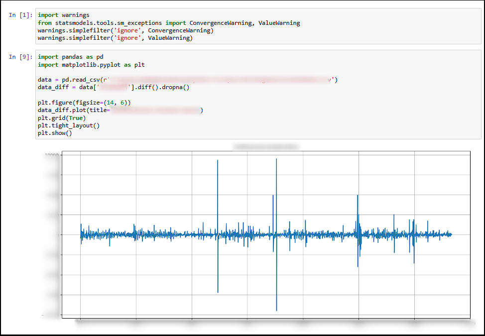
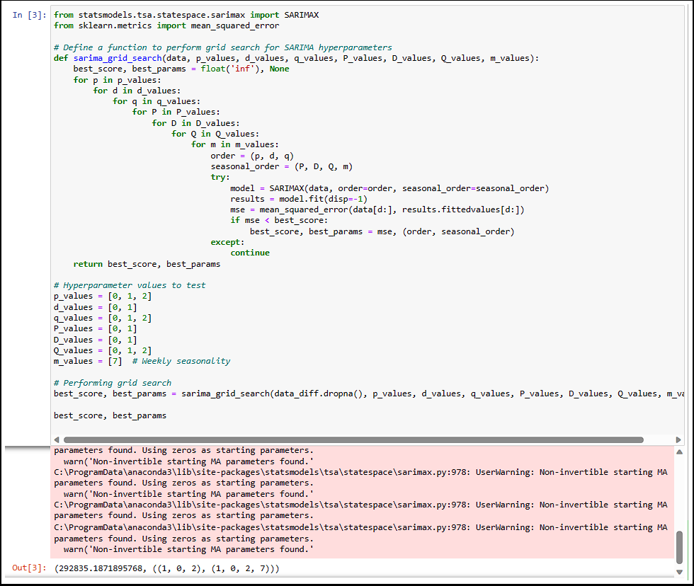
Since clear trends are visible in the data over time, a SARIMA model is required (as opposed to a standard ARIMA model). The next step involves finding the optimal parameters for SARIMA using a grid search function:

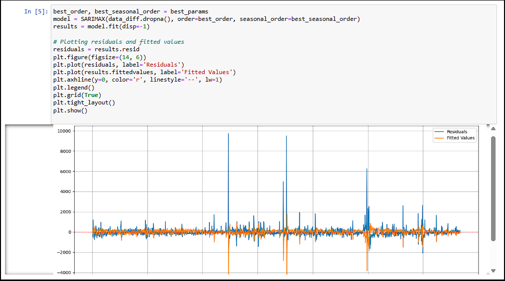
Using the best parameters derived from the grid search, I fitted the SARIMA model. I plotted the residuals and fitted values for visual inspection. As seen below, both are centered around the red dashed line at zero, indicating a mean of zero. While there is some remaining seasonality in the residuals, the results are satisfactory for this use case.

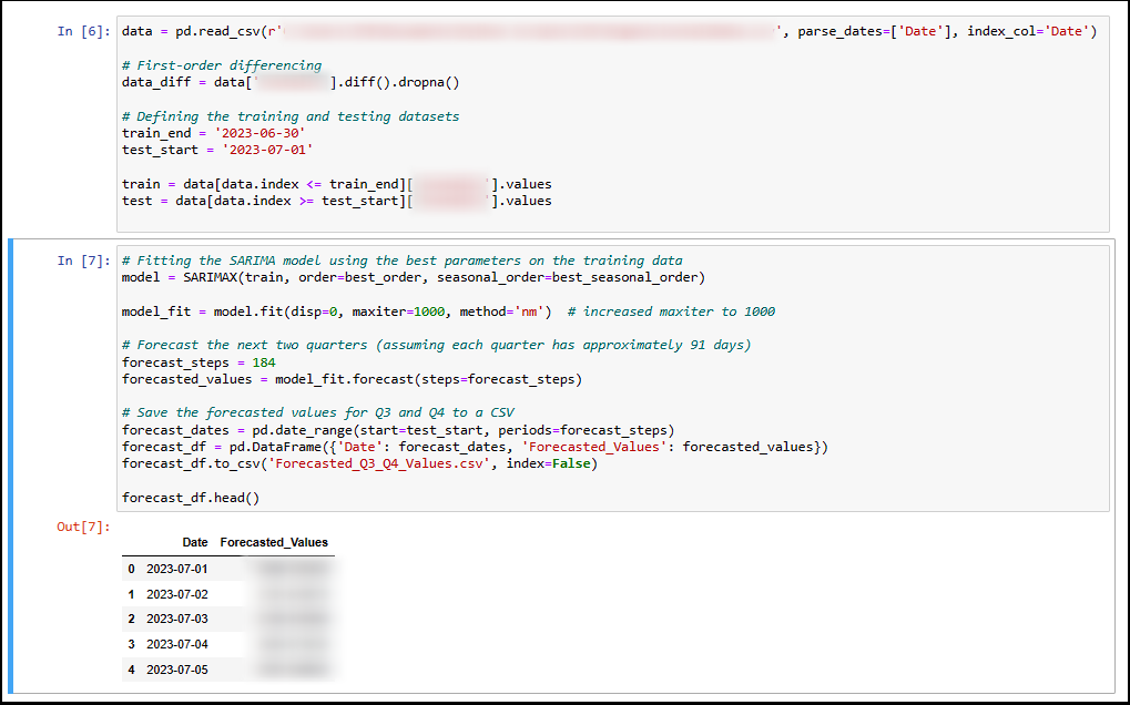
Next, I reloaded the dataset. Based on previous results, I performed first-order differencing and then defined the training and testing datasets. Finally, I fitted the SARIMA model using the optimized parameters and forecasted the next two quarters, saving the output to a CSV file.

3. Results

Due to the sensitive nature of the data used in this project, I cannot share the specific underlying information. However, the chart below compares the real values obtained for the first month of Q3 (July) against my projected results.

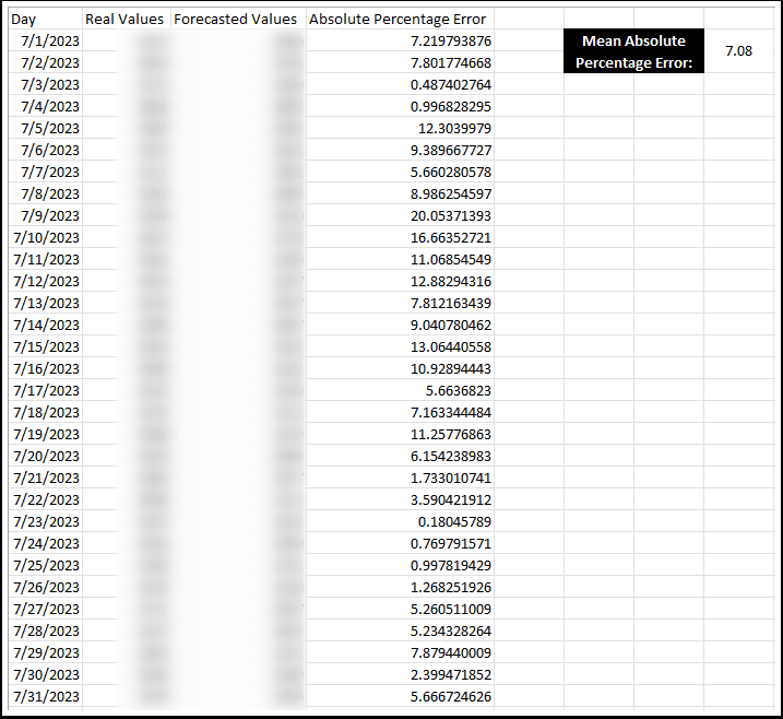
The Mean Absolute Percentage Error (MAPE) for the forecasted installs in July is approximately 7.08%. This indicates that, on average, the forecasted values deviated by only 7.08% from the actual values, resulting in an model accuracy of roughly 93%.